Homogeneous Coordinates and Matrix Derivation of Basic Geometric Transformations in Two-Dimensional Graphics

Homogeneous Coordinates#

"Homogeneous coordinates are one of the important means of computer graphics. It can be used to distinguish between vectors and points, and is also easier to use for affine (linear) geometric transformations." - F.S. Hill, JR.

As mentioned in the quote, the biggest advantage of homogeneous coordinates is that they can distinguish between coordinates and vectors.

Simply put, in a regular Cartesian coordinate system (or Cartesian coordinate system), (x_A, y_A) can represent point A, or it can be used to represent vector $\vec{oA}$ . This ambiguous representation is not conducive to accurately abstracting descriptions for computers.

Homogeneous coordinates solve this problem by elevating n dimensions to n+1 dimensions.

We can add an additional variable w to the end of a 2D Cartesian coordinate to form a 2D homogeneous coordinate. Therefore, a point (X,Y) becomes (x,y,w) in homogeneous coordinates, and we have

X = x/w

Y = y/w

In homogeneous coordinates,

Describing a point A is represented as (x_A, y_A, 1)
Describing a vector $\vec{oA}$ is represented as (x_A, y_A, 0)

Try substituting w=1,0 into x/w, and you will understand why 1 represents a point (position) and 0 represents a vector (direction).

In addition, it is also convenient for operations such as vector addition.

Of course, in addition to describing vectors and points, the introduction of homogeneous coordinates also facilitates the description of geometric transformations (linear transformations).

For example, if we don't use homogeneous coordinates to represent a 2D translation, it would look like this:

Basic Geometric Transformations in 2D#

2D geometric transformations can be roughly divided into the following five categories: translation, scaling, rotation, reflection, and shear.

1. Translation#

Describes the transformation from point (x, y) to (x + dx, y + dy).

By introducing homogeneous coordinates, it can be expressed as (x, y, 1) transformed to (x + dx, y + dy, 1).

At this point, linear transformation can be used as a tool to describe the transformation process. After introducing the transformation matrix, the problem becomes solving the transformation matrix.

Given:

\begin{pmatrix} a & b & c \\ d & e & f \\ g & h & i \end{pmatrix} \begin{pmatrix} x \\ y \\ 1 \end{pmatrix} = \begin{pmatrix} x + dx \\ y + dy \\ 1 \end{pmatrix}

We have:

\begin{cases} ax + by + c = x + dx \\ dx + ey + f = y + dy \\ gx + hy + i = 1 \end{cases}

The solution for the transformation matrix is:

\begin{pmatrix} 1 & 0 & dx \\ 0 & 1 & dy \\ 0 & 0 & 1 \end{pmatrix}

So, mathematically, we can use this transformation matrix to describe the translation process.

2. Scaling#

Describes the transformation from point (x, y) to (sx * x, sy * y), where sx and sy are constants.

By introducing homogeneous coordinates, it can be expressed as (x, y, 1) transformed to (sx * x, sy * y, 1).

By introducing the transformation matrix:

Given:

\begin{pmatrix} a & b & c \\ d & e & f \\ g & h & i \end{pmatrix} \begin{pmatrix} x \\ y \\ 1 \end{pmatrix} = \begin{pmatrix} sx * x \\ sy * y \\ 1 \end{pmatrix}

We have:

\begin{cases} ax + by + c = sx * x \\ dx + ey + f = sy * y \\ gx + hy + i = 1 \end{cases}

The solution for the transformation matrix is:

\begin{pmatrix} sx & 0 & 0 \\ 0 & sy & 0 \\ 0 & 0 & 1 \end{pmatrix}

3. Rotation#

Explanation of rotation requires the introduction of the unit circle.

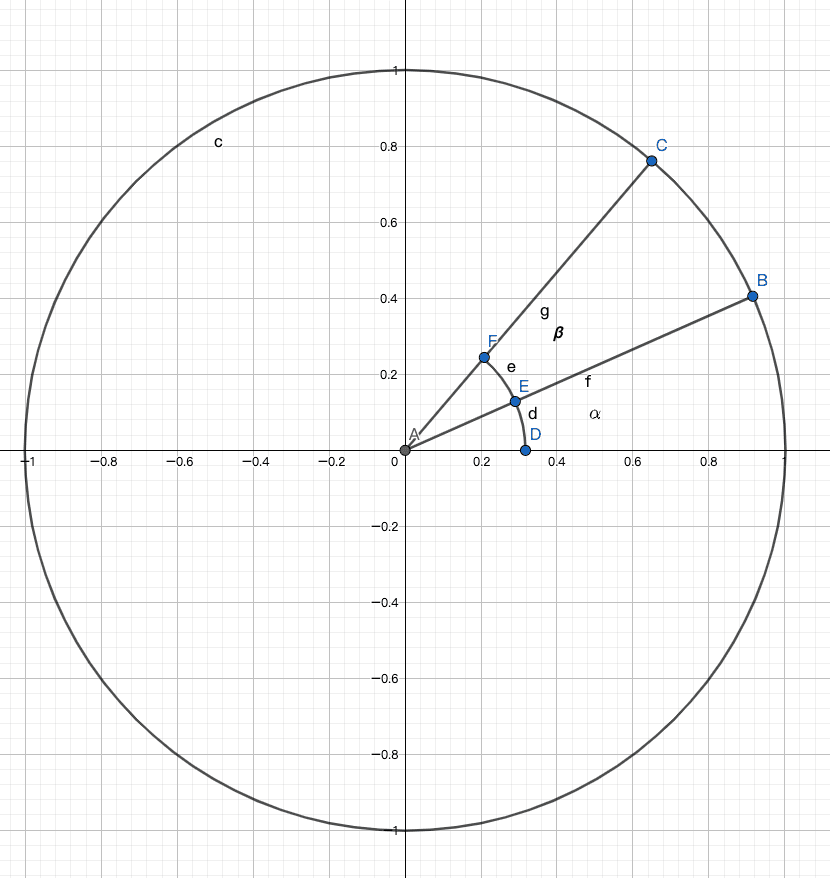
As shown in the figure, point B is rotated to point C, and the angle between AB and the X-axis is α, and the angle between AC and AB is β.

Then the coordinates of point B can be represented as (cosα, sinα), and the coordinates of point C are (cos(α + β), sin(α + β)).

Expanding the coordinates of point C, we have C as (cosα cosβ - sinα sinβ, sinα cosβ + cosα sinβ).

Let the coordinates of point B be (x, y), then the coordinates of point C are (x cosβ - y sinβ, y cosβ + x sinβ).

By introducing homogeneous coordinates, it can be expressed as (x, y, 1) transformed to (x cosβ - y sinβ, y cosβ + x sinβ, 1).

By introducing the transformation matrix:

Given:

\begin{pmatrix} a & b & c \\ d & e & f \\ g & h & i \end{pmatrix} \begin{pmatrix} x \\ y \\ 1 \end{pmatrix} = \begin{pmatrix} xcosβ - ysinβ \\ ycosβ + xsinβ \\ 1 \end{pmatrix}

We have:

\begin{cases} ax + by + c = xcosβ - ysinβ \\ dx + ey + f = ycosβ + xsinβ \\ gx + hy + i = 1 \end{cases}

The solution for the transformation matrix is:

\begin{pmatrix} cosβ & -sinβ & 0 \\ sinβ & cosβ & 0 \\ 0 & 0 & 1 \end{pmatrix}

4. Reflection#

In mathematics, reflection is a mapping that transforms an object into its mirror image. To reflect a plane figure, a "mirror line" is needed (the axis of reflection), and for reflection in three-dimensional space, a plane is used as the mirror.

If we go by the quote, reflection can be divided into reflection based on the X-axis and reflection based on the Y-axis. However, there is also the concept of central reflection (point reflection).

Reflection based on the X-axis#

Describes the transformation from point (x, y) to (x, -y).

Given:

\begin{pmatrix} a & b & c \\ d & e & f \\ g & h & i \end{pmatrix} \begin{pmatrix} x \\ y \\ 1 \end{pmatrix} = \begin{pmatrix} x \\ -y \\ 1 \end{pmatrix}

We have:

\begin{cases} ax + by + c = x \\ dx + ey + f = -y \\ gx + hy + i = 1 \end{cases}

The solution for the transformation matrix is:

\begin{pmatrix} 1 & 0 & 0 \\ 0 & -1 & 0 \\ 0 & 0 & 1 \end{pmatrix}

Reflection based on the Y-axis#

Describes the transformation from point (x, y) to (-x, y).

Given:

\begin{pmatrix} a & b & c \\ d & e & f \\ g & h & i \end{pmatrix} \begin{pmatrix} x \\ y \\ 1 \end{pmatrix} = \begin{pmatrix} -x \\ y \\ 1 \end{pmatrix}

We have:

\begin{cases} ax + by + c = -x \\ dx + ey + f = y \\ gx + hy + i = 1 \end{cases}

The solution for the transformation matrix is:

\begin{pmatrix} -1 & 0 & 0 \\ 0 & 1 & 0 \\ 0 & 0 & 1 \end{pmatrix}

Reflection based on the point (p, q)#

Describes the transformation from point (x, y) to (2p-x, 2q-y).

Given:

\begin{pmatrix} a & b & c \\ d & e & f \\ g & h & i \end{pmatrix} \begin{pmatrix} x \\ y \\ 1 \end{pmatrix} = \begin{pmatrix} 2p-x \\ 2q-y \\ 1 \end{pmatrix}

We have:

\begin{cases} ax + by + c = 2p-x \\ dx + ey + f = 2q-y \\ gx + hy + i = 1 \end{cases}

The solution for the transformation matrix is:

\begin{pmatrix} -1 & 0 & 2p \\ 0 & -1 & 2q \\ 0 & 0 & 1 \end{pmatrix}

5. Shear#

The definition can be seen in the figure, which is actually like the distortion of a shape in a certain direction. The range of α and β is [0, 90°).

Shear dependent on the y-axis#

Describes the transformation from point (x, y) to (x + y * tanα, y).

Given:

\begin{pmatrix} a & b & c \\ d & e & f \\ g & h & i \end{pmatrix} \begin{pmatrix} x \\ y \\ 1 \end{pmatrix} = \begin{pmatrix} x+y.tanα \\ y \\ 1 \end{pmatrix}

We have:

\begin{cases} ax + by + c = x+y.tanα \\ dx + ey + f = y \\ gx + hy + i = 1 \end{cases}

The solution for the transformation matrix is:

\begin{pmatrix} 1 & tanα & 0 \\ 0 & 1 & 0 \\ 0 & 0 & 1 \end{pmatrix}

Shear dependent on the x-axis#

Describes the transformation from point (x, y) to (x, y + x * tanβ).

Given:

\begin{pmatrix} a & b & c \\ d & e & f \\ g & h & i \end{pmatrix} \begin{pmatrix} x \\ y \\ 1 \end{pmatrix} = \begin{pmatrix} x \\ y + x.tanβ \\ 1 \end{pmatrix}

We have:

\begin{cases} ax + by + c = x \\ dx + ey + f = y + x.tanβ \\ gx + hy + i = 1 \end{cases}

The solution for the transformation matrix is:

\begin{pmatrix} 1 & 0 & 0 \\ tanβ & 1 & 0 \\ 0 & 0 & 1 \end{pmatrix}